Contents
- check whether the timing of the sequence is correct
- prepare export
- plots and displays
- plot entire interpolated wave forms -- good for debugging of gaps, jumps,
- trajectory calculation
- very optional slow step, but useful for testing during development e.g. for the real TE, TR or for staying within slewrate limits
% we define here a really crude True-FISP a.k.a. bSSFP sequence
% there is no user control for TR/TE, you just specify the ADC time and the
% RF parameters and the rest is calculated to find the fastest posible
% timing. The sequence intensively uses the extended trapezoid
% functionality to achieve near-optimal timing. Due to the requirement for
% splitting the sequence into blocks the TR is increased by approximately
% 40-60 us (rfDeadTime+adcDeadTime) in comparison to the true minimum TR

% set system limits
% had to slow down ramps and increase adc_duration to avoid stimulation
sys = mr.opts('MaxGrad',30,'GradUnit','mT/m',...
    'MaxSlew',140,'SlewUnit','T/m/s',...
    'rfRingdownTime', 20e-6, 'rfDeadTime', 100e-6, ...
    'adcDeadTime', 20e-6);

seq=mr.Sequence(sys);              % Create a new sequence object
fov=220e-3; Nx=256; Ny=256;     % Define FOV and resolution


% ADC duration (controls TR/TE)
adc_dur=2560; %us

% RF parameters
alpha=40; % deg
thick=4; %mm
rf_dur=600; % us
rf_apo=0.5;
rf_bwt=1.5;

% Create 'alpha' degree slice selection pulse and gradient
[rf, gz, gzReph] = mr.makeSincPulse(alpha*pi/180,'Duration',rf_dur*1e-6,...
    'SliceThickness',thick*1e-3,'apodization',rf_apo,'timeBwProduct',rf_bwt,'system',sys);

% Define other gradients and ADC events
deltak=1/fov;
gx = mr.makeTrapezoid('x','FlatArea',Nx*deltak,'FlatTime',adc_dur*1e-6,'system',sys);
adc = mr.makeAdc(Nx,'Duration',gx.flatTime,'Delay',gx.riseTime,'system',sys);
gxPre = mr.makeTrapezoid('x','Area',-gx.area/2,'system',sys);
phaseAreas = ((0:Ny-1)-Ny/2)*deltak;

% now we have to reshuffle gradients to achieve a half-way optimal timing
% new gz will consist of two parts:
% 1: slice refocusing from the previous TR followed by slice selection
%    including the plato an a small bit of the ramp-down
% 2: the remainder of the ramp-down and the slice refocusing for the next TR
gz_parts=mr.splitGradientAt(gz,mr.calcDuration(rf));
gz_parts(1).delay=mr.calcDuration(gzReph);
gz_1=mr.addGradients({gzReph,gz_parts(1)},'system',sys);
[rf,~]=mr.align('right',rf,gz_1);
gz_parts(2).delay=0;
gzReph.delay=mr.calcDuration(gz_parts(2));
gz_2=mr.addGradients({gz_parts(2),gzReph},'system',sys);

% new gr will consist of two parts:
% 1: prephaser followed by a part of the read gradient including the
%    beginning of the ramp-down
% 2: the remainer of the ramp-down and the second "prephaser"
gx_parts=mr.splitGradientAt(gx,ceil(mr.calcDuration(adc)/sys.gradRasterTime)*sys.gradRasterTime);
gx_parts(1).delay=mr.calcDuration(gxPre);
gx_1=mr.addGradients({gxPre,gx_parts(1)},'system',sys);
adc.delay=adc.delay+mr.calcDuration(gxPre); % we cannot use mr.align here because the adc duration maz be not aligneed to the grad raster
gx_parts(2).delay=0;
gxPre.delay=mr.calcDuration(gx_parts(2));
gx_2=mr.addGradients({gx_parts(2),gxPre},'system',sys);

% Calculate timing
%pe_dur=min(max(tp2(end),tpr1(end-2)),max(tp(end-3),tpr2(end)));
gxPre.delay=0; % otherwise duration below is misreported
%pe_dur=max(mr.calcDuration(gz_2),mr.calcDuration(gxPre)+gx.riseTime);
pe_dur=mr.calcDuration(gx_2);

% adjust delays to align objects
%gz_1.delay=max(mr.calcDuration(gx_2)-rf.delay,0);
gz_1.delay=max(mr.calcDuration(gx_2)-rf.delay+rf.ringdownTime,0); % this rf.ringdownTime is needed to center the ADC and the gradient echo in the center of RF-RF period

rf.delay=rf.delay+gz_1.delay;

% finish timing calculation
TR=mr.calcDuration(gz_1)+mr.calcDuration(gx_1);
TE=TR/2;

% alpha / 2 preparation: shorter TR and half-angle, no PE, no RO
% create 0.5*alpha prep pulse
rf05=rf;
rf05.signal=0.5*rf.signal;
seq.addBlock(rf05,gz_1,mr.makeLabel('SET','ONCE', 1)); % we also label the few following blocks as preparing to exclude them if the sequence is repeated
% the following delay calculation fails for agressive sequence timing
prepDelay=mr.makeDelay(round((TR/2-mr.calcDuration(gz_1))/sys.gradRasterTime)*sys.gradRasterTime); % I know this round() is not 100% correct
gx_1_1=mr.makeExtendedTrapezoidArea('x',0,gx_2.first,-gx_2.area,sys);
gyPre_2 = mr.makeTrapezoid('y','Area',phaseAreas(end),'Duration',pe_dur,'system',sys); % last PE step (in case of repetitions)
seq.addBlock(mr.align('left',prepDelay,gz_2,gyPre_2,'right',gx_1_1));
seq.addBlock(mr.makeLabel('SET','ONCE', 0)); % remove preparing block label

% Loop over phase encodes and define sequence blocks
for i=1:Ny
    rf.phaseOffset=pi*mod(i,2);
    adc.phaseOffset=pi*mod(i,2);

    gyPre_1 = mr.scaleGrad(gyPre_2,-1); % undo previous PE step
    gyPre_2 = mr.makeTrapezoid('y','Area',phaseAreas(i),'Duration',pe_dur,'system',sys); % current PE step

    seq.addBlock(rf,gz_1, gyPre_1, gx_2);
    seq.addBlock(gx_1,gyPre_2, gz_2,adc);
end
% finish the x-grad shape
seq.addBlock(gx_2,mr.makeLabel('SET','ONCE', 2)); % we also label this block as the exit block, which excludes it from all but last repetitions if the sequence is repeated

% check that the calculated TR was reached
% alpha / 2 prep takes 4 blocks
assert(TR==(mr.calcDuration(seq.getBlock(5))+mr.calcDuration(seq.getBlock(6))));

fprintf('Sequence ready\n');
fprintf('TR=%03f ms  TE=%03f ms\n', TR*1e3, TE*1e3);
Sequence ready
TR=4.740000 ms  TE=2.370000 ms
check whether the timing of the sequence is correct
[ok, error_report]=seq.checkTiming;

if (ok)
    fprintf('Timing check passed successfully\n');
else
    fprintf('Timing check failed! Error listing follows:\n');
    fprintf([error_report{:}]);
    fprintf('\n');
end
Timing check passed successfully
prepare export
seq.setDefinition('FOV', [fov fov thick*1e-3]);
seq.setDefinition('Name', 'trufi');

seq.write('trufi.seq')       % Write to pulseq file

%seq.install('siemens');
plots and displays
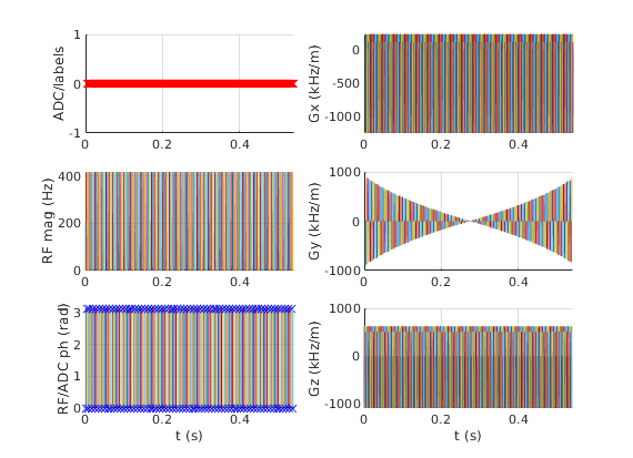
seq.plot('timeDisp','us');

plot entire interpolated wave forms -- good for debugging of gaps, jumps,
etc, but is relatively slow
%gw=seq.gradient_waveforms();
%figure; plot(gw'); % plot the entire gradient waveform
gw_data=seq.waveforms_and_times();
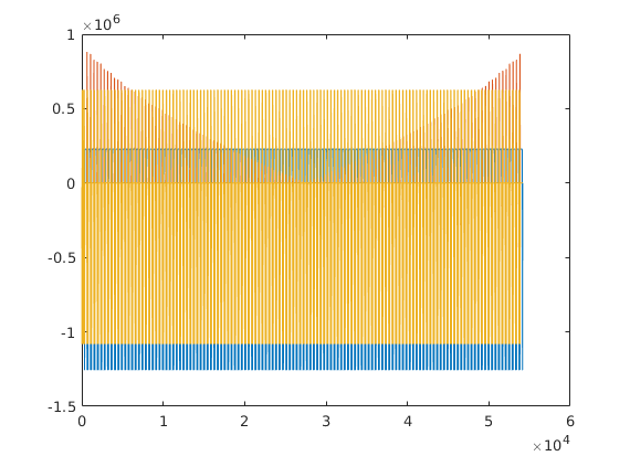
figure; plot(gw_data{1}(1,:),gw_data{1}(2,:),gw_data{2}(1,:),gw_data{2}(2,:),gw_data{3}(1,:),gw_data{3}(2,:)); % plot the entire gradient waveform
title('gradient waveforms');

trajectory calculation
[ktraj_adc, t_adc, ktraj, t_ktraj, t_excitation, t_refocusing] = seq.calculateKspacePP();

% plot k-spaces

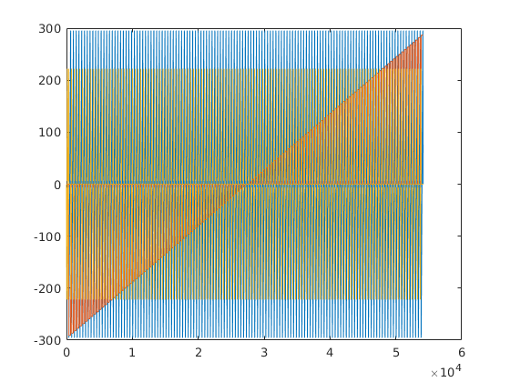
figure; plot(t_ktraj,ktraj'); title('k-space components as functions of time'); % plot the entire k-space trajectory
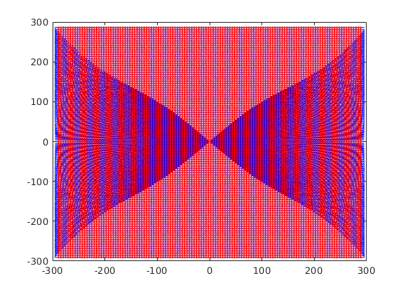
figure; plot(ktraj(1,:),ktraj(2,:),'b',...
             ktraj_adc(1,:),ktraj_adc(2,:),'r.'); % a 2D plot
title('2D k-space');


very optional slow step, but useful for testing during development e.g. for the real TE, TR or for staying within slewrate limits
rep = seq.testReport;
fprintf([rep{:}]);
Number of blocks: 516
Number of events:
   RF:      257
   Gx:      514
   Gy:      513
   Gz:      514
   ADC:     256
Sequence duration: 1.216560s
TE: 0.002370s
TR: 0.004740s
Flip angle: 20.00°
Flip angle: 40.00°
Unique k-space positions (a.k.a. columns, rows, etc): 256
Unique k-space positions (a.k.a. columns, rows, etc): 256
Dimensions: 2
   Spatial resolution: 0.86 mm
   Spatial resolution: 0.86 mm
Repetitions/slices/contrasts: 1  range: [1 1]
   65536 k-space position(s) repeated 1 times
Cartesian encoding trajectory detected
Block timing check passed successfully
Max. Gradient: 1276596 Hz/m == 29.98 mT/m
Max. Gradient: 1003135 Hz/m == 23.56 mT/m
Max. Gradient: 1109375 Hz/m == 26.06 mT/m
Max. Slew Rate: 5.80271e+09 Hz/m/s == 136.29 T/m/s
Max. Slew Rate: 5.9596e+09 Hz/m/s == 139.98 T/m/s
Max. Slew Rate: 5.68182e+09 Hz/m/s == 133.45 T/m/s
Max. Absolute Gradient: 1966390 Hz/m == 46.19 mT/m
Max. Absolute Slew Rate: 1.00733e+10 Hz/m/s == 236.60 T/m/s