Create a TSE sequence and export for execution

The Sequence class provides functionality to create magnetic resonance sequences (MRI or NMR) from basic building blocks.

This provides an implementation of the open file format for MR sequences described here: http://pulseq.github.io/specification.pdf

This example performs the following steps:

Create slice selective RF pulse for imaging.
Create readout gradient and phase encode strategy.
Loop through phase encoding and generate sequence blocks.
Write the sequence to an open file format suitable for execution on a scanner.

Juergen Hennig <juergen.hennig@uniklinik-freiburg.de>
Maxim Zaitsev  <maxim.zaitsev@uniklinik-freiburg.de>

Instantiation and gradient limits
Sequence events
Base gradients
Slice selection
Readout gradient
Phase encoding
split gradients and recombine into blocks
Define sequence blocks
new single-function call for trajectory calculation
plot k-spaces
Write to file

Instantiation and gradient limits

The system gradient limits can be specified in various units mT/m, Hz/cm, or Hz/m. However the limits will be stored internally in units of Hz/m for amplitude and Hz/m/s for slew. Unspecificied hardware parameters will be assigned default values.

dG=250e-6;
system = mr.opts('MaxGrad', 30, 'GradUnit', 'mT/m', ...
    'MaxSlew', 170, 'SlewUnit', 'T/m/s', 'rfRingdownTime', 100e-6, ...
    'rfDeadTime', 100e-6, 'adcDeadTime', 10e-6);

A new sequence object is created by calling the class constructor.

seq=mr.Sequence(system);

Sequence events

Some sequence parameters are defined using standard MATLAB variables

fov=256e-3;
Ny_pre=8;
Nx=128; Ny=128; necho=Ny/2+Ny_pre; Nslices=1;
rflip=180;
if (numel(rflip)==1), rflip=rflip+zeros([1 necho]); end
sliceThickness=5e-3;
TE=12e-3; TR=2000e-3;
TEeff=60e-3;
k0=round(TEeff/TE);
PEtype='linear';

readoutTime = 6.4e-3 + 2*system.adcDeadTime;
tEx=2.5e-3;
tExwd=tEx+system.rfRingdownTime+system.rfDeadTime;
tRef=2e-3;
tRefwd=tRef+system.rfRingdownTime+system.rfDeadTime;
tSp=0.5*(TE-readoutTime-tRefwd);
tSpex=0.5*(TE-tExwd-tRefwd);
fspR=1.0;
fspS=0.5;

rfex_phase=pi/2; % MZ: we need to maintain these as variables because we will overwrtite phase offsets for multiple slice positions
rfref_phase=0;

Base gradients

Slice selection

Key concepts in the sequence description are blocks and events. Blocks describe a group of events that are executed simultaneously. This hierarchical structure means that one event can be used in multiple blocks, a common occurrence in MR sequences, particularly in imaging sequences.

First, the slice selective RF pulses (and corresponding slice gradient) are generated using the makeSincPulse function. Gradients are recalculated such that their flattime covers the pulse plus the rfdead- and rfringdown- times.

flipex=90*pi/180;
[rfex, gz] = mr.makeSincPulse(flipex,system,'Duration',tEx,...
    'SliceThickness',sliceThickness,'apodization',0.5,'timeBwProduct',4,'PhaseOffset',rfex_phase);
GSex = mr.makeTrapezoid('z',system,'amplitude',gz.amplitude,'FlatTime',tExwd,'riseTime',dG);
% plotPulse(rfex,GSex);

flipref=rflip(1)*pi/180;
[rfref, gz] = mr.makeSincPulse(flipref,system,'Duration',tRef,...
    'SliceThickness',sliceThickness,'apodization',0.5,'timeBwProduct',4,'PhaseOffset',rfref_phase,'use','refocusing');
GSref = mr.makeTrapezoid('z',system,'amplitude',GSex.amplitude,'FlatTime',tRefwd,'riseTime',dG);
% plotPulse(rfref,GSref);

AGSex=GSex.area/2;
GSspr = mr.makeTrapezoid('z',system,'area',AGSex*(1+fspS),'duration',tSp,'riseTime',dG);
GSspex = mr.makeTrapezoid('z',system,'area',AGSex*fspS,'duration',tSpex,'riseTime',dG);

Readout gradient

To define the remaining encoding gradients we need to calculate the $k$ -space sampling. The Fourier relationship

$\Delta k = \frac{1}{FOV}$

Therefore the area of the readout gradient is $n\Delta k$ .

deltak=1/fov;
kWidth = Nx*deltak;

GRacq = mr.makeTrapezoid('x',system,'FlatArea',kWidth,'FlatTime',readoutTime,'riseTime',dG);
adc = mr.makeAdc(Nx,'Duration',GRacq.flatTime-40e-6, 'Delay', 20e-6);%,'Delay',GRacq.riseTime);
GRspr = mr.makeTrapezoid('x',system,'area',GRacq.area*fspR,'duration',tSp,'riseTime',dG);
GRspex = mr.makeTrapezoid('x',system,'area',GRacq.area*(1+fspR),'duration',tSpex,'riseTime',dG);


AGRspr=GRspr.area;%GRacq.area/2*fspR;
AGRpreph = GRacq.area/2+AGRspr;%GRacq.area*(1+fspR)/2;
GRpreph = mr.makeTrapezoid('x',system,'Area',AGRpreph,'duration',tSpex,'riseTime',dG);

Phase encoding

To move the $k$ -space trajectory away from 0 prior to the readout a prephasing gradient must be used. Furthermore rephasing of the slice select gradient is required.

%[PEorder,Ny] = myTSE_PEorder(Ny,necho,k0,PEtype);
%nex=floor(Ny/necho);
%pe_steps=(1:(necho*nex))-0.5*necho*nex-1;
%if 0==mod(necho,2)
%    pe_steps=circshift(pe_steps,[0,-round(nex/2)]); % for odd number of echoes we have to apply a shift to avoid a contrast jump at k=0
%end
%PEorder=reshape(pe_steps,[nex,necho])';
nex=1;
PEorder=((-Ny_pre):Ny)';
phaseAreas = PEorder*deltak;

split gradients and recombine into blocks

lets start with slice selection....

GS1times=[0 GSex.riseTime];
GS1amp=[0 GSex.amplitude];
GS1 = mr.makeExtendedTrapezoid('z','times',GS1times,'amplitudes',GS1amp);

GS2times=[0 GSex.flatTime];
GS2amp=[GSex.amplitude GSex.amplitude];
GS2 = mr.makeExtendedTrapezoid('z','times',GS2times,'amplitudes',GS2amp);

GS3times=[0 GSspex.riseTime GSspex.riseTime+GSspex.flatTime GSspex.riseTime+GSspex.flatTime+GSspex.fallTime];
GS3amp=[GSex.amplitude GSspex.amplitude GSspex.amplitude GSref.amplitude];
GS3 = mr.makeExtendedTrapezoid('z','times',GS3times,'amplitudes',GS3amp);

GS4times=[0 GSref.flatTime];
GS4amp=[GSref.amplitude GSref.amplitude];
GS4 = mr.makeExtendedTrapezoid('z','times',GS4times,'amplitudes',GS4amp);

GS5times=[0 GSspr.riseTime GSspr.riseTime+GSspr.flatTime GSspr.riseTime+GSspr.flatTime+GSspr.fallTime];
GS5amp=[GSref.amplitude GSspr.amplitude GSspr.amplitude 0];
GS5 = mr.makeExtendedTrapezoid('z','times',GS5times,'amplitudes',GS5amp);

GS7times=[0 GSspr.riseTime GSspr.riseTime+GSspr.flatTime GSspr.riseTime+GSspr.flatTime+GSspr.fallTime];
GS7amp=[0 GSspr.amplitude GSspr.amplitude GSref.amplitude];
GS7 = mr.makeExtendedTrapezoid('z','times',GS7times,'amplitudes',GS7amp);

% and now the readout gradient....

GR3=GRpreph;%GRspex;

GR5times=[0 GRspr.riseTime GRspr.riseTime+GRspr.flatTime GRspr.riseTime+GRspr.flatTime+GRspr.fallTime];
GR5amp=[0 GRspr.amplitude GRspr.amplitude GRacq.amplitude];
GR5 = mr.makeExtendedTrapezoid('x','times',GR5times,'amplitudes',GR5amp);

GR6times=[0 readoutTime];
GR6amp=[GRacq.amplitude GRacq.amplitude];
GR6 = mr.makeExtendedTrapezoid('x','times',GR6times,'amplitudes',GR6amp);

GR7times=[0 GRspr.riseTime GRspr.riseTime+GRspr.flatTime GRspr.riseTime+GRspr.flatTime+GRspr.fallTime];
GR7amp=[GRacq.amplitude GRspr.amplitude GRspr.amplitude 0];
GR7 = mr.makeExtendedTrapezoid('x','times',GR7times,'amplitudes',GR7amp);


% and filltimes
tex=GS1.t(end)+GS2.t(end)+GS3.t(end);
tref=GS4.t(end)+GS5.t(end)+GS7.t(end)+readoutTime;
tend=GS4.t(end)+GS5.t(end);
tETrain=tex+necho*tref+tend;
TRfill=(TR-Nslices*tETrain)/Nslices;
% round to gradient raster
TRfill=system.gradRasterTime * round(TRfill / system.gradRasterTime);
if TRfill<0, TRfill=1e-3;
    disp(strcat('Warning!!! TR too short, adapted to include all slices to : ',num2str(1000*Nslices*(tETrain+TRfill)),' ms'));
else
    disp(strcat('TRfill : ',num2str(1000*TRfill),' ms'));
end
delayTR = mr.makeDelay(TRfill);
delayEnd = mr.makeDelay(5);

TRfill :1127.82 ms

Define sequence blocks

Next, the blocks are put together to form the sequence

for kex=1:nex % MZ: we start at 0 to have one dummy
    for s=1:Nslices
        rfex.freqOffset=GSex.amplitude*sliceThickness*(s-1-(Nslices-1)/2);
        rfref.freqOffset=GSref.amplitude*sliceThickness*(s-1-(Nslices-1)/2);
        rfex.phaseOffset=rfex_phase-2*pi*rfex.freqOffset*mr.calcRfCenter(rfex); % align the phase for off-center slices
        rfref.phaseOffset=rfref_phase-2*pi*rfref.freqOffset*mr.calcRfCenter(rfref); % dito

        seq.addBlock(GS1);
        seq.addBlock(GS2,rfex);
        seq.addBlock(GS3,GR3);
        %GS4.first=GS4f;
        %GS4.first=GS3.last;
        for kech=1:necho,
            if (kex>0)
                phaseArea=phaseAreas(kech,kex);
            else
                phaseArea=0;
            end
            GPpre = mr.makeTrapezoid('y',system,'Area',phaseArea,'Duration',tSp,'riseTime',dG);
            GPrew = mr.makeTrapezoid('y',system,'Area',-phaseArea,'Duration',tSp,'riseTime',dG);
            seq.addBlock(GS4,rfref);
            seq.addBlock(GS5,GR5,GPpre);
            if (kex>0)
                seq.addBlock(GR6,adc);
            else
                seq.addBlock(GR6);
            end
            seq.addBlock(GS7,GR7,GPrew);
            %GS4.first=GS7.last;
        end
        seq.addBlock(GS4);
        seq.addBlock(GS5);
        seq.addBlock(delayTR);
    end
end

seq.addBlock(delayEnd);

new single-function call for trajectory calculation

[ktraj_adc, ktraj, t_excitation, t_refocusing] = seq.calculateKspace();

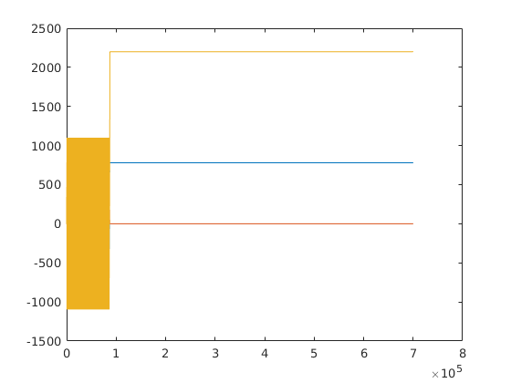
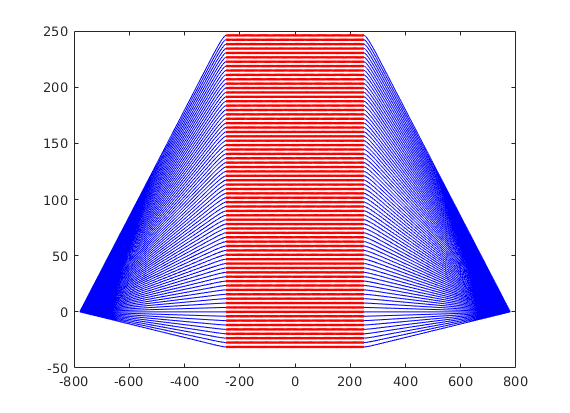
plot k-spaces

figure; plot(ktraj'); % plot the entire k-space trajectory
figure; plot(ktraj(1,:),ktraj(2,:),'b',...
             ktraj_adc(1,:),ktraj_adc(2,:),'r.'); % a 2D plot

Write to file

% The sequence is written to file in compressed form according to the file
% format specification using the |write| method.
seq.write('haste.seq')

Display the first few lines of the output file s=fileread('myTSE.seq'); disp(s(1:300))

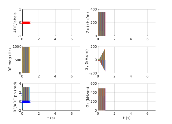
seq.plot();

% seq.install('siemens');