Contents

% this is an experimentaal high-performance EPI sequence
% which uses split gradients to overlap blips with the readout
% gradients combined with ramp-samping

seq=mr.Sequence();         % Create a new sequence object
fov=256e-3; Nx=64; Ny=Nx;  % Define FOV and resolution
thickness=4e-3;            % slice thinckness
Nslices=3;

pe_enable=1;               % a flag to quickly disable phase encoding (1/0) as needed for the delay calibration
ro_os=1;                   % oversampling factor (in contrast to the product sequence we don't really need it)
readoutTime=4.2e-4;        % this controls the readout bandwidth
partFourierFactor=1;       % partial Fourier factor: 1: full sampling 0: start with ky=0

% Set system limits
lims = mr.opts('MaxGrad',32,'GradUnit','mT/m',...
    'MaxSlew',130,'SlewUnit','T/m/s',...
    'rfRingdownTime', 30e-6, 'rfDeadtime', 100e-6);

% Create fat-sat pulse
B0=2.89; % 1.5 2.89 3.0
sat_ppm=-3.45;
sat_freq=sat_ppm*1e-6*B0*lims.gamma;
rf_fs = mr.makeGaussPulse(110*pi/180,'system',lims,'Duration',8e-3,...
    'bandwidth',abs(sat_freq),'freqOffset',sat_freq);
gz_fs = mr.makeTrapezoid('z',lims,'delay',mr.calcDuration(rf_fs),'Area',1/1e-4); % spoil up to 0.1mm

% Create 90 degree slice selection pulse and gradient
[rf, gz, gzReph] = mr.makeSincPulse(pi/2,'system',lims,'Duration',3e-3,...
    'SliceThickness',thickness,'apodization',0.5,'timeBwProduct',4);

% define the output trigger to play out with every slice excitatuion
trig=mr.makeDigitalOutputPulse('osc0','duration', 100e-6); % possible channels: 'osc0','osc1','ext1'

% Define other gradients and ADC events
deltak=1/fov;
kWidth = Nx*deltak;

% Phase blip in shortest possible time
blip_dur = ceil(2*sqrt(deltak/lims.maxSlew)/10e-6/2)*10e-6*2; % we round-up the duration to 2x the gradient raster time
% the split code below fails if this really makes a trpezoid instead of a triangle...
gy = mr.makeTrapezoid('y',lims,'Area',-deltak,'Duration',blip_dur); % we use negative blips to save one k-space line on our way towards the k-space center
%gy = mr.makeTrapezoid('y',lims,'amplitude',deltak/blip_dur*2,'riseTime',blip_dur/2, 'flatTime', 0);

% readout gradient is a truncated trapezoid with dead times at the beginnig
% and at the end each equal to a half of blip_dur
% the area between the blips should be defined by kWidth
% we do a two-step calculation: we first increase the area assuming maximum
% slewrate and then scale down the amlitude to fix the area
extra_area=blip_dur/2*blip_dur/2*lims.maxSlew; % check unit!;
gx = mr.makeTrapezoid('x',lims,'Area',kWidth+extra_area,'duration',readoutTime+blip_dur);
actual_area=gx.area-gx.amplitude/gx.riseTime*blip_dur/2*blip_dur/2/2-gx.amplitude/gx.fallTime*blip_dur/2*blip_dur/2/2;
gx.amplitude=gx.amplitude/actual_area*kWidth;
gx.area = gx.amplitude*(gx.flatTime + gx.riseTime/2 + gx.fallTime/2);
gx.flatArea = gx.amplitude*gx.flatTime;

% calculate ADC
% we use ramp sampling, so we have to calculate the dwell time and the
% number of samples, which are will be qite different from Nx and
% readoutTime/Nx, respectively.
adcDwellNyquist=deltak/gx.amplitude/ro_os;
% round-down dwell time to 100 ns
adcDwell=floor(adcDwellNyquist*1e7)*1e-7;
adcSamples=floor(readoutTime/adcDwell/4)*4; % on Siemens the number of ADC samples need to be divisible by 4
% MZ: no idea, whether ceil,round or floor is better for the adcSamples...
adc = mr.makeAdc(adcSamples,'Dwell',adcDwell,'Delay',blip_dur/2);
% realign the ADC with respect to the gradient
time_to_center=adc.dwell*((adcSamples-1)/2+0.5); % I've been told that Siemens samples in the center of the dwell period
adc.delay=round((gx.riseTime+gx.flatTime/2-time_to_center)*1e6)*1e-6; % we adjust the delay to align the trajectory with the gradient. We have to aligh the delay to 1us
% this rounding actually makes the sampling points on odd and even readouts
% to appear misalligned. However, on the real hardware this misalignment is
% much stronger anyways due to the grdient delays

% FOV positioning requires alignment to grad. raster... -> TODO

% split the blip into two halves and produnce a combined synthetic gradient
gy_parts = mr.splitGradientAt(gy, blip_dur/2, lims);
%gy_blipup=gy_parts(1);
%gy_blipdown=gy_parts(2);
%gy_blipup.delay=gx.riseTime+gx.flatTime+gx.fallTime-blip_dur/2;
%gy_blipdown.delay=0;
[gy_blipup, gy_blipdown]=mr.align('right',gy_parts(1),'left',gy_parts(2),gx);
gy_blipdownup=mr.addGradients({gy_blipdown, gy_blipup}, lims);

% pe_enable support
gy_blipup.waveform=gy_blipup.waveform*pe_enable;
gy_blipdown.waveform=gy_blipdown.waveform*pe_enable;
gy_blipdownup.waveform=gy_blipdownup.waveform*pe_enable;

% phase encoding and partial Fourier

Ny_pre=round(partFourierFactor*Ny/2-1); % PE steps prior to ky=0, excluding the central line
Ny_post=round(Ny/2+1); % PE lines after the k-space center including the central line
Ny_meas=Ny_pre+Ny_post;

% Pre-phasing gradients
gxPre = mr.makeTrapezoid('x',lims,'Area',-gx.area/2);
gyPre = mr.makeTrapezoid('y',lims,'Area',Ny_pre*deltak);
[gxPre,gyPre,gzReph]=mr.align('right',gxPre,'left',gyPre,gzReph);
% relax the PE prepahser to reduce stimulation
gyPre = mr.makeTrapezoid('y',lims,'Area',gyPre.area,'Duration',mr.calcDuration(gxPre,gyPre,gzReph));
gyPre.amplitude=gyPre.amplitude*pe_enable;

% Define sequence blocks
for s=1:Nslices
    seq.addBlock(rf_fs,gz_fs);
    rf.freqOffset=gz.amplitude*thickness*(s-1-(Nslices-1)/2);
    seq.addBlock(rf,gz,trig);
    seq.addBlock(gxPre,gyPre,gzReph);
    for i=1:Ny_meas
        if i==1
            seq.addBlock(gx,gy_blipup,adc); % Read the first line of k-space with a single half-blip at the end
        elseif i==Ny_meas
            seq.addBlock(gx,gy_blipdown,adc); % Read the last line of k-space with a single half-blip at the beginning
        else
            seq.addBlock(gx,gy_blipdownup,adc); % Read an intermediate line of k-space with a half-blip at the beginning and a half-blip at the end
        end
        gx.amplitude = -gx.amplitude;   % Reverse polarity of read gradient
    end
end

check whether the timing of the sequence is correct

[ok, error_report]=seq.checkTiming;

if (ok)
    fprintf('Timing check passed successfully\n');
else
    fprintf('Timing check failed! Error listing follows:\n');
    fprintf([error_report{:}]);
    fprintf('\n');
end

Timing check passed successfully

do some visualizations

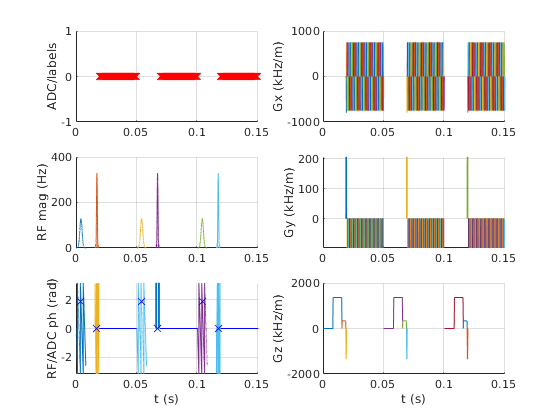
seq.plot();             % Plot sequence waveforms

% trajectory calculation
[ktraj_adc, ktraj, t_excitation, t_refocusing, t_adc] = seq.calculateKspace();

% plot k-spaces
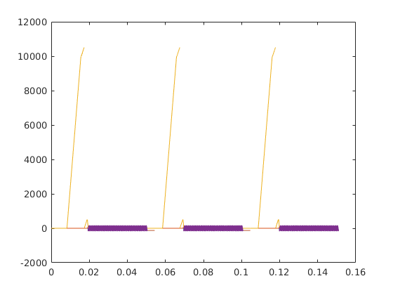
time_axis=(1:(size(ktraj,2)))*lims.gradRasterTime;
figure; plot(time_axis, ktraj'); % plot the entire k-space trajectory
hold on; plot(t_adc,ktraj_adc(1,:),'.'); % and sampling points on the kx-axis
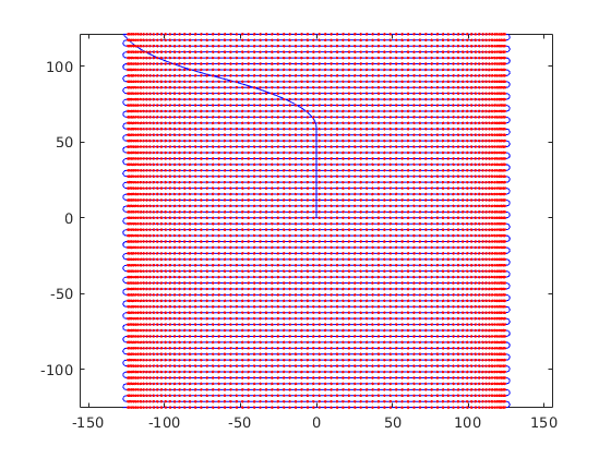
figure; plot(ktraj(1,:),ktraj(2,:),'b'); % a 2D plot
axis('equal'); % enforce aspect ratio for the correct trajectory display
hold on;plot(ktraj_adc(1,:),ktraj_adc(2,:),'r.'); % plot the sampling points
%axis off;

return;

another manual pretty plot option

lw=1;
gw=seq.gradient_waveforms();
ofs=2.05*max(abs(gw(:)));
% plot the entire gradient waveforms
figure; plot(time_axis, gw(3,:)+2*ofs,'Color',[0,0.5,0.3],'LineWidth',lw);
hold on; plot(time_axis, gw(2,:)+1*ofs,'r','LineWidth',lw);
plot(time_axis, gw(1,:),'b','LineWidth',lw);
t_adc_gr=t_adc+0.5*seq.gradRasterTime; % we have to shift the time axis because it is otherwise adpted to the k-space, which is a one-sided integration of the trajeectory
gwr_adc=interp1(time_axis,gw(1,:),t_adc_gr);
plot(t_adc_gr,gwr_adc,'b.','MarkerSize',3*lw); % and sampling points on the kx-axis
xlim([-0.03*time_axis(end),1.03*time_axis(end)]);
%axis off;

new higher-performabce trajectory calculation

[ktraj_adc1, t_adc1, ktraj1, t_ktraj1, t_excitation1, t_refocusing1] = seq.calculateKspacePP();

% plot k-spaces
figure; plot(t_ktraj1, ktraj1'); % plot the entire k-space trajectory
hold on; plot(t_adc1,ktraj_adc1(1,:),'.'); % and sampling points on the kx-axis
figure; plot(ktraj1(1,:),ktraj1(2,:),'b'); % a 2D plot
axis('equal'); % enforce aspect ratio for the correct trajectory display
hold on;plot(ktraj_adc1(1,:),ktraj_adc1(2,:),'r.'); % plot the sampling points

compare both

figure; plot(time_axis, ktraj');
hold on; plot(t_ktraj1, ktraj1','-.');

prepare the sequence output for the scanner

seq.setDefinition('FOV', [fov fov thickness]);
seq.setDefinition('Name', 'epi');

seq.write('epi_rs.seq');

% seq.install('siemens');

% seq.sound(); % simulate the seq's tone

very optional slow step, but useful for testing during development e.g. for the real TE, TR or for staying within slewrate limits

rep = seq.testReport;
fprintf([rep{:}]); % as for January 2019 TR calculation fails for fat-sat

Published with MATLAB® R2020a