Read a sequence into MATLAB

The Sequence class provides an implementation of the open file format for MR sequences described here: http://pulseq.github.io/specification.pdf

This example demonstrates parsing an MRI sequence stored in this format, accessing sequence parameters and visualising the sequence.

Contents

Read a sequence file

A sequence can be loaded from the open MR file format using the read method. seq_name='trufi.seq';

seq_name='../examples/gre.seq';
seq=mr.Sequence();
seq.read(seq_name);

sanity check to see if the reading and writing are consistent

seq.write('read_test.seq'); system(['diff -s -u ' seq_name ' read_test.seq'],'-echo');

Access sequence parameters and blocks

Parameters defined with in the [DEFINITIONS] section of the sequence file are accessed with the getDefinition method. These are user-specified definitions and do not effect the execution of the sequence.

scanId=seq.getDefinition('Scan_ID')

scanId =

     []

Sequence blocks are accessed with the getBlock method. As shown in the output the first block is a selective excitation block and contains an RF pulse and gradient and on the z-channel.

b1 = seq.getBlock(1)

b1 = 

  struct with fields:

           rf: [1×1 struct]
           gx: []
           gy: []
           gz: [1×1 struct]
          adc: []
        delay: []
    gexternal: [1×1 struct]

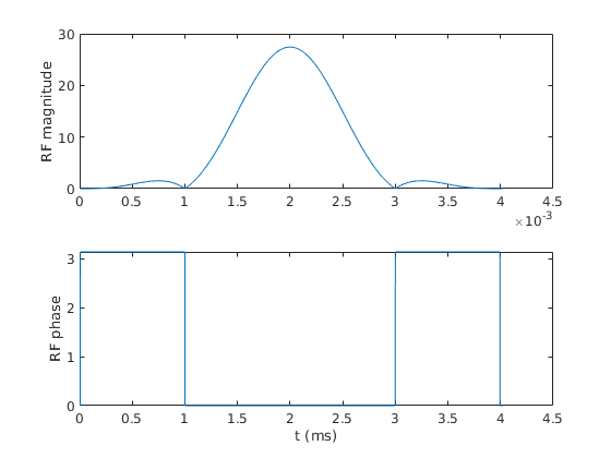
Further information about each event can be obtained by accessing the appropriate fields of the block struct. In particular, the complex RF signal is stored in the field signal.

rf=b1.rf

figure;
subplot(211);
plot(rf.t,abs(rf.signal));
ylabel('RF magnitude');
subplot(212);
plot(1e3*rf.t,angle(rf.signal))
ylabel('RF phase'); xlabel('t (ms)');

rf = 

  struct with fields:

            type: 'rf'
          signal: [4020×1 double]
               t: [4020×1 double]
           delay: 1.0000e-04
      freqOffset: 0
     phaseOffset: 0
        deadTime: 0
    ringdownTime: 0

The next three blocks contain: three gradient events; a delay; and readout gradient with ADC event, each with corresponding fields defining the details of the events.

b2 = seq.getBlock(2);
b3 = seq.getBlock(3);
b4 = seq.getBlock(4);
b2.gx
b3.delay
b4.adc

ans = 

  struct with fields:

         type: 'trap'
      channel: 'x'
    amplitude: -6.4748e+04
     riseTime: 2.0000e-05
     flatTime: 0.0020
     fallTime: 2.0000e-05
        delay: 0
         area: -128.2001
     flatArea: -126.9051


ans = 

  struct with fields:

     type: 'delay'
    delay: 1.2000e-04


ans = 

  struct with fields:

     numSamples: 64
          dwell: 1.0000e-04
          delay: 1.0000e-05
     freqOffset: 0
    phaseOffset: 0
       deadTime: 0
           type: 'adc'

Plot the sequence

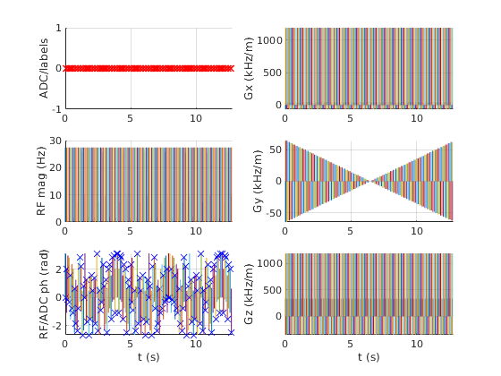
Visualise the sequence using the plot method of the class. This creates a new figure and shows ADC, RF and gradient events. The axes are linked so zooming is consistent. In this example, a simple gradient echo sequence for MRI is displayed.

seq.plot()

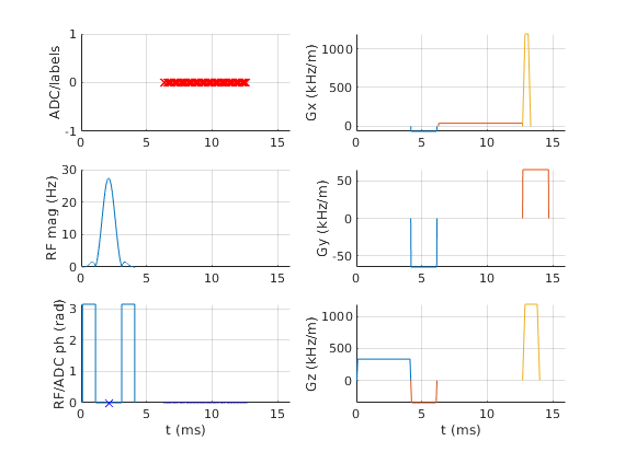
The details of individual pulses are not well-represented when the entire sequence is visualised. Interactive zooming is helpful here. Alternatively, a time range can be specified. An additional parameter also allows the display units to be changed for easy reading. Further, the handle of the created figure can be returned if required.

fig=seq.plot('TimeRange',[0 16e-3],'timeDisp','ms')

fig = 

  Figure (3) with properties:

      Number: 3
        Name: ''
       Color: [0.9400 0.9400 0.9400]
    Position: [1320 1278 560 420]
       Units: 'pixels'

  Use GET to show all properties

Modifying sequence blocks

In addition to loading a sequence and accessing sequence blocks, blocks can be modified. In this example, a Hamming window is applied to the first RF pulse of the sequence and the flip angle is changed to 45 degrees. The remaining RF pulses are unchanged.

rf2=rf;
duration=rf2.t(end);
t=rf2.t-duration/2;                                 % Centre time about 0
alpha=0.5;
BW=4/duration;                                      % time bandwidth product = 4
window = (1.0-alpha+alpha*cos(2*pi*t/duration));    % Hamming window
signal = window.*sinc(BW*t);

% Normalise area to achieve 2*pi rotation
signal=signal./(seq.rfRasterTime*sum(real(signal)));

% Scale to 45 degree flip angle
rf2.signal=signal.*45/360;

b1.rf=rf2;
seq.setBlock(1,b1);

second check to see what we have changed

seq.write('read_test2.seq'); system(['diff -s -u ' seq_name ' read_test2.seq'],'-echo');

The amplitude of the first rf pulse is reduced due to the reduced flip-angle. Notice the reduction is not exactly a factor of two due to the windowing function.

amp1_in_Hz = max(abs(seq.getBlock(1).rf.signal))
amp2_in_Hz = max(abs(seq.getBlock(6).rf.signal))

amp1_in_Hz =

  122.8179


amp2_in_Hz =

   27.4293

Published with MATLAB® R2020a